Trapezium Velocity Profile

A typical way to control robotic joints is to use a trapezoidal speed profile, which is quite similar to the profiles you’d get by driving your car: acceleration , constant speed , and deceleration.

Imagine a vehicle running to its target. Instead of rushing and bumping into the end point, the vehicle must accelerate and keep running at a constant speed , and before reaching the goal, it will start decelerating and get to the end safely. That is the general idea of Trapezium Velocity Profile which we applied to the motion of Franka robot.

The Trapezium Velocity Profile is widely used in the industry, and the profile is constructed with two main input parameters:

1. The desired target speed of end-effector travel
2. The acceleration of the end-effector.( it will be mirrored to create deceleration period)

The middle section is scaled according to the travel distance to keep the end-effector at a constant speed.

To implement the Trapezium Velocity Profile, firstly we need to discretise the path into a number of small, equally sized unit. The ideal size of each unit is dx which is calculated by dx = acceleration * dt**2.

There are two case that we considered while applying the profile. The first case is that the length of the path is long enough for the end-effector to reach the target speed. The middle sectiond is scaled along the time axis accordingly.

Based on the two input parameters, the profile will be constructed:

The end stage time = target_speed / acceleration
The end stage displacement = end_stage_time * target_speed / 2
The mid stage displacement = path_length - 2 * end_stage_displacement
The mid stage time = mid_stage_displacement / target_speed
The total time = end_stage_time * 2 + mid_stage_time

Then creating a time list using 0->Total time in steps of dt:

time_list = np.arange(start=0, stop=total_time, step=dt)
np.reshape(time_list, (np.shape(time_list)[0], 1))

The dt variable is fixed by the control loop running the libfranka control loop. Therefore, it cannot be changed locally from 0.05 seconds in this trajectory generator.

A list of speeds is then calculated by applying this time list and the parameters calculated earlier, speed graph is sampled to create list to go with time list:

speed_values = []
c = (0 - (-acc) * time_list[-1]) # c is the calculated intercept for the deceleration period)
for t in time_list:
    if t <= end_stage_t:
        # acceleration period
        speed_values.append(acc * t)

    elif t >= end_stage_t + mid_stage_t:
        # deceleration stage
        speed_values.append(-acc * t + c)

    elif t > end_stage_t:
        # constant speed at target speed
        speed_values.append(target_speed)

The original discretised path list is now sampled using the speed list. For each speed, the corresponding number of samples in the path list is calculated (speed_value * dt / dx)```` and these sampled points are stored in a new list of new_marker:

new_marker = np.hstack((smooth_path[smooth_path_idx], speed_values[i]))

Finally the trajectory will be return as a vertical stack in the form of[start position, end position, speed information] by:

trajectory = np.vstack((trajectory, new_marker))

On the other hand, when the traveling path is not far enough , there isn’t enough time to accelerate, reach constant velocity and then decelerate. The profile will then simply become triangular.

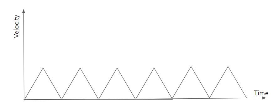
In this case the profile is still useful becasue it decrease the speed of the motion as a whole. However, the target speed will be calculated differently if path lenth is shorter than minimum path length (which is target_speed ** 2 / acceleration):

``target_speed = np.sqrt(path_length * acceleration)``

Documentation

Functions:

apply_trapezoid_vel(path, acceleration=1, max_speed=1): Takes a path (currently only a start/end point (straight line), and returns a discretised trajectory of the path controlled by a trapezium velocity profile generated by the input parameters.

Parameters:

path-list of 2 points in 3D space.

acceleration-Acceleration and deceleration of trapezium profile.

max_speed-Target maximum speed of the trapezium profile.

Return:

Trajectory as numpy array.

discretise(point_1, point_2, dx) Takes a straight line and divides it into smaller defined length segments.

Parameters:

point_1 – First point in 3D space.

point_2 – Second point in 3D space.

dx – Distance between points in discretised line.

Return:

Numpy array of discretised line.

discretise_path(move, dx) Discretise a moves path using object defined dx for unit.

Parameters:

move – List of points path goes through.

dx – Displacement between two points on the target discretised path.

Returns:

Discretised path as numpy array